In practice, over 128 values, the variations are spread out over 35 to 45 values. That is to say a report/ratio S/B from approximately 35 with 40dB.

Figure 3 is obtained by carrying out a polar transformation
= > rectangular, with teta constant (method 2, to see further). Then, the
rectangular transform " fft2 " produces the coefficients of Fourrier.
The columns are increasing according to teta. The lines
are increasing according to R.
It is noticed that information is primarily at the highest frequencies.
With the reading of this figure, one could believe that the values are distributed in a horizontal way:
| The values are distributed primarily on the high and
low edges. Thus, the quantity of information present on each line varies
much according to N°of the line. On the other hand, the quantity of
information present on each column varies little according to N°of
the column.
One deduces from it that the columns contain more information than the lines! The information contained on the iris seems more to be distributed more in a circular way. But it as should be noticed as the average perimeter of an iris is much more significant than its ray. It can thus be carrying much more information. |
One should not forget the role of the polar = > rectangular transform. It is possible that it is here, responsible for a such distribution.


For more speed, one can use a simpler filtering and more running, with
filters RII or RIF and a convolution 2D. The filter will be thus a high
pass one, with a high frequency cut-off and a significant attenuation.
However, no precise value imposes the choice of a particular filter.
Here an example based on a filtering band suppressor centered in average frequencies. The lowest frequencies are so little significant here that filtering in average region has the effect of a low-pass filtering.
Figure 1: FFT 2D of the image of a complete eye. Figure 2: FFT 2D of the filtered image. One notices the standardization of low and intermediate frequency.The implementation of this filter is carried out, under Matlab, with the command < medfilt2(source) >, which carries out a local approximation with an interpolation of the type " nearest ". One obtains a standardization of the values in low and average tape as well as a general attenuation of the noise.
The use of the wavelets is described after. One is interested here only in the results and not in the methods.
Within the framework of the multiresolution analysis, filters are deduced
from the wavelets. These filters are (generally) per pair High-Pass (here
G(z)) / Low-Pass (here H(z)). The residue (A1(x)) is obtained by applying
the filter Low-Pass (H(z)). This residue corresponds to the remainder after
a decomposition by a wavelet.
The process can be iterated, on the condition of carrying out a decimation
(resolution divided by 2) between the filters. Below : a decomposition
of order 3:

Denoising can be done on orders 1 or 2 only.
Below : Pictures denoised with such method.
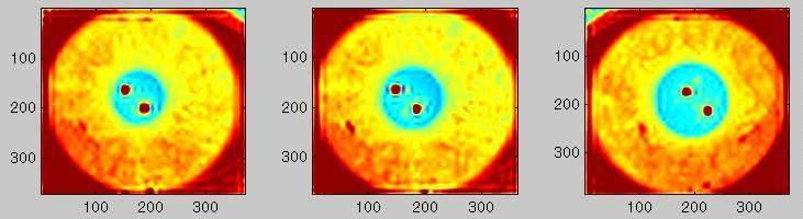
Approximation at order 2 (low-pass residue)
The principal problem is the side effect, that leads to small waves
on the extremities.
But the main parameters of the iris are well kept.
| Return | Synopsis | Continuation |
